>model
income=constant+educatn
>estimate
Data for the following results were selected according to:
sex$='Male'
Dep Var: INCOME N: 104 Multiple R: 0.473796 Squared multiple R: 0.224482
Adjusted squared multiple R: 0.216879 Standard error of estimate: 14.528751
Effect
Coefficient Std Error Std Coef
Tolerance t P(2 Tail)
CONSTANT
4.879179 3.962622 0.000000
. 1.23130 0.22104
EDUCATN
5.371633 0.988578 0.473796
1.000000 5.43370 0.00000
Analysis of Variance
Source
Sum-of-Squares df Mean-Square
F-ratio P
Regression
6232.282646 1 6232.282646 29.525044
0.000000
Residual
2.15306E+04 102 211.084616
-------------------------------------------------------------------------------
Durbin-Watson
D Statistic 1.968
First
Order Autocorrelation 0.012
>
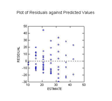
Plot
of Residuals against Predicted Values
>estimate
Data for the following results were selected according to:
sex$='Male'
Dep
Var: INCOME N: 104 Multiple R: 0.476472
Squared multiple R: 0.227025
Adjusted
squared multiple R: 0.195794 Standard error of estimate: 14.723041
Effect
Coefficient Std Error Std Coef
Tolerance t P(2 Tail)
CONSTANT
13.388889 3.470254 0.000000
. 3.85819 0.00020
HSGRA
7.841880 4.195332 0.232359
0.505263 1.86919 0.06455
SOMCO
15.905229 4.979329 0.359977
0.614778 3.19425 0.00188
COGRA
17.548611 5.058721 0.387521
0.625668 3.46898 0.00078
GRADE
24.825397 5.246531 0.518600
0.650000 4.73177 0.00001
Analysis of Variance
Source
Sum-of-Squares df Mean-Square
F-ratio P
Regression
6302.888552 4 1575.722138
7.269166 0.000036
Residual
2.14600E+04 99 216.767928
-------------------------------------------------------------------------------
Durbin-Watson
D Statistic 1.933
First
Order Autocorrelation 0.028
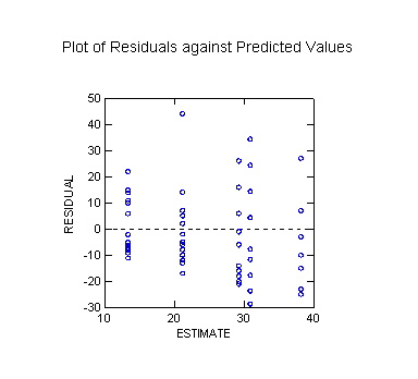
Plot
of Residuals against Predicted Values
>estimate
Data for the following results were selected according to:
sex$='Male'
Model
contains no constant
Note the inflated R-Square when constant is not
included. This is called non-centered R-Square and should
not be used as a measure of fit.
Dep
Var: INCOME N: 104 Multiple R: 0.876517
Squared multiple R: 0.768283
Adjusted
squared multiple R: 0.758920 Standard error of estimate: 14.723041
Effect
Coefficient Std Error Std Coef
Tolerance t P(2 Tail)
HSDRO
13.388889 3.470254 0.186657
1.000000 3.85819 0.00020
HSGRA
21.230769 2.357573 0.435674
1.000000 9.00535 0.00000
SOMCO
29.294118 3.570862 0.396889
1.000000 8.20365 0.00000
COGRA
30.937500 3.680760 0.406639
1.000000 8.40519 0.00000
GRADE
38.214286 3.934898 0.469844
1.000000 9.71163 0.00000
Analysis of Variance
Source
Sum-of-Squares df Mean-Square
F-ratio P
Regression
7.11530E+04 5 1.42306E+04 65.648987
0.000000
Residual
2.14600E+04 99 216.767928
-------------------------------------------------------------------------------
Durbin-Watson
D Statistic 1.933
First
Order Autocorrelation 0.028
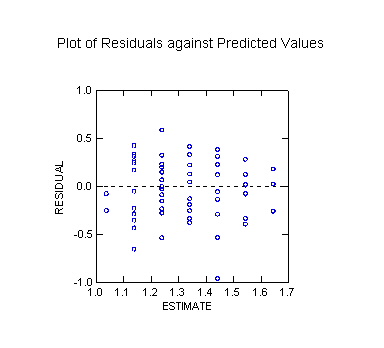
Plot of Residuals against Predicted Values

>estimate
Data for the following results were selected according to:
sex$='Male'
Dep
Var: L10INC N: 104 Multiple R: 0.462675
Squared multiple R: 0.214068
Adjusted
squared multiple R: 0.206362 Standard error of estimate: 0.282933
Effect
Coefficient Std Error Std Coef
Tolerance t P(2 Tail)
CONSTANT
0.936115 0.077168 0.000000
. 12.13085 0.00000
EDUCATN
0.101473 0.019252 0.462675
1.000000 5.27088 0.00000
Analysis of Variance
Source
Sum-of-Squares df Mean-Square
F-ratio P
Regression
2.223991 1 2.223991
27.782171 0.000001
Residual
8.165203 102 0.080051
-------------------------------------------------------------------------------
***
WARNING ***
Case
237 is an outlier (Studentized
Residual = -3.646594)
Durbin-Watson
D Statistic 1.805
First
Order Autocorrelation 0.093
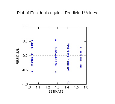
Plot of Residuals against Predicted Values
>estimate
Data for the following results were selected according to:
sex$='Male'
Dep Var: L10INC N: 104 Multiple R: 0.492572 Squared multiple R: 0.242627
Adjusted squared multiple R: 0.212026 Standard error of estimate: 0.281922
Effect
Coefficient Std Error Std Coef
Tolerance t P(2 Tail)
CONSTANT
1.033201 0.066450 0.000000
. 15.54866 0.00000
HSGRA
0.248897 0.080334 0.381243
0.505263 3.09830 0.00253
SOMCO
0.376642 0.095346 0.440662
0.614778 3.95028 0.00015
COGRA
0.381972 0.096866 0.436039
0.625668 3.94330 0.00015
GRADE
0.511031 0.100462 0.551855
0.650000 5.08679 0.00000
Analysis of Variance
Source
Sum-of-Squares df Mean-Square
F-ratio P
Regression
2.520699 4 0.630175
7.928745 0.000014
Residual
7.868495 99 0.079480
-------------------------------------------------------------------------------
***
WARNING ***
Case
237 is an outlier (Studentized
Residual = -3.643266)
Durbin-Watson
D Statistic 1.764
First
Order Autocorrelation 0.113
Plot of Residuals against Predicted Values
>REM
End of command batch file D:\MYDOCS\YS209\INCXED.SYC