SOCI209 - Module 5 - Multiple Regression & the General Linear Model
1. Need for Models With More Than One Independent Variable
1. Motivations for Multiple Regression Analysis
The 2 principal motivations for models with more than one independent variable
are:
-
to make the predictions of the model more precise by adding other factors
believed to affect the dependent variable to reduce the proportion of error
variance associated with SSE; for example
-
in a model explaining prestige of current occupation as a function of years
of education, add SES of family of origin and IQ
-
in a study the sale prices of homes in a county, include as many characteristics
of the house that can affect the price (such as heated area, land area,
age of the house, number of bathrooms, etc.) to obtain the best fitting
model, in order to derive estimates ^Yh of the values of houses
in the county (for tax purposes) that are as accurate as possible
-
to support a causal theory by eliminating potential sources of spuriousness.
This is sometimes called the elaboration model.; for example
-
in a model of socioeconomic success as a function of SES of family of origin,
add IQ of subject to control for a possible inflated effect of SES that
overestimates childhood environmental influences on adult outcome
The second motivation is very important for scientific applications of
regression analysis. It is discussed further in the next section.
2. Supporting a Causal Statement by Eliminating Alternative Hypotheses
Theories about social phenomena are made up of causal statements.
A causal statement or law is "a statement or proposition
in a theory which says that there exist environments ... in which a change
in the value of one variable is associated with a change in the value of
another variable and can produce this change without any change in other
variables in the environment" (Stinchcombe, Arthur. 1968. Constructing
Social Theories, p. 31). Such a causal statement can be represented
schematically as

where Y is the dependent variable and X the independent variable.
One of the requirements to support or refute a causal theory is to ascertain
nonspuriousness. This means eliminating the possibility that
one or more other variables (say Z and W) affect both X and Y and thereby
produce an apparent association between X and Y that is spuriously attributed
to a causal influence of X on Y. The mechanism of spurious association
is shown in the following picture:

Multiple regression analysis can be used to ascertain nonspuriousness by
adding variables explicitly to the regression model to eliminate alternative
hypotheses on the source of the relationship between X and Y. The
effectiveness of this strategy depends on the design of the study:
-
with experimental data (in which the values of some of the X variables
are deliberately set by the experimenter) ascertaining nonspuriousness
is effective, since the value of the "treatment" has been deliberately
dissociated (through random assignment) from the values of the other independent
variables characterizing the elements, as in the following picture

-
with observational data one can try to establish non-spuriousness by including
explicit measures of the variables suspected of causing a spurious association
in a multiple regression model. If including these variables (say
Z and W) renders the effect of X on Y non-significant, this is a clue that
the association between X and Y is not causal (i.e., is spurious).
This method is called covariance control; its principle is illustrated
in the following picture

With observational data the task of ascertaining nonspuriousness remains
open-ended, as it is never possible to prove that all potential
sources of spuriousness have been controlled. In the context of regression
analysis, spuriousness is called
specification bias. Specification
bias is a more general and continuous notion than spuriousness. The
idea is that if a regression model of Y on X excludes a variable that is
both
associated with X and a cause of Y (the model is then called
misspecified)
the estimated association of Y with X will be inflated (or, conversely,
deflated) relative to its true value. The regression estimator, in
a sense, falsely "attributes" to X a causal influence that is in reality
due to the omitted variable(s).
2. Yule's Study of Pauperism (1899)
1. The First Modern Multiple Regression Analysis
The use of multiple regression analysis as a means of controlling for possible
confounding factors that may spuriously produce an apparent relationship
between two variables was first proposed by G. Udny Yule in the late 1890s.
In a pathbreaking 1899 paper "An Investigation into the Causes of Changes
in Pauperism in England, chiefly in the last Two Intercensal Decades" Yule
investigated the effect of a change in the ratio of the poor receiving
relief outside as opposed to inside the poorhouses (the "out-relief ratio")
on change in pauperism (poverty rate) in British unions. (Unions
are British administrative units.) This was a hot topic of policy
debate in Great Britain at the time. Charles Booth had argued that
increasing the proportion of the poor receiving relief outside the poorhouses
did not increase pauperism in a union. Using correlation coefficients
(a then entirely novel technique that had been just developed by his colleague
and mentor Karl Pearson), Yule had discovered that there was a strong bivariate
association between change in the out-relief ratio and change in pauperism,
contrary to Booth's impression. In the 1899 paper Yule uses multiple
regression to confirm the relationship between pauperism and out-relief
by controlling for other possible causes of the apparent association, specifically
change in proportion of the old (to control for the greater incidence of
poverty among the elderly) and change in population (using population increase
in a union as an indicator of prosperity). The 1899 paper is the
first published use of multiple regression analysis. It is hard to
improve on Yule's description of the logic of the method. (On this
episode in the history of statistics see Stigler 1986, pp. 345-361.)
Yule's argument is that (using modern notation) in the estimated simple
regression model
^Y = b0 + b1X1
where ^Y is change in pauperism and X1 is change in the proportion
of out-relief , the association between Y and X1 measured by
b1 confounds the direct effect of X1 on Y with the
common association of both Y and X1 with other variables ("economic
and social changes") that are not explicitly included in the model.
By contrast, in the multiple regression model
^Y = b0 + b1X1 + b2X2
+ b3X3
where X2 measures change in proportion of the elderly and X3
measures change in population, the (partial) regression coefficient b1
now measures the estimated effect of X1 on Y when the other
factors included in the model are kept constant. The possibility
that b1 contains a spurious component due to the joint association
of Y with X1, X2, and X3 is now excluded,
since X2 and X3 are explicitly included in the model
(i.e., "controlled").
2. Applying the Elaboration Model to Yule's Data
The technique of "testing" the coefficient of a variable X1
for spuriousness by introducing in the model additional variables X2,
X3, etc., measuring potential confounding factors is called
the elaboration model. It is an effective and widely used
strategy to conduct a regression analysis, and to present the results.
Thus, as remarked above, the standard tabular presentation of regression
results is often based on the elaboration model.
These points are illustrated by a replication of Yule's (1899) analysis
for 32 unions in the London metropolitan area. The dependent variable is
change in pauperism (labeled PAUP). The predictor of interest is
change in the out-relief ratio (OUTRATIO). The control variables
are change in the proportion of the old (PROPOLD) and change in population
(POP). The following exhibits show Yule's (1899) original results
and the replication using the elaboration model strategy, in which each
control variable is added to the model in turn.
The first model, a simple regression of PAUP on OUTRATIO, shows a significant
positive effect of OUTRATIO on PAUP. In the second model, including
PROPOLD in addition to OUTRATIO, the coefficient of OUTRATIO remains positive
and highly significant. PROPOLD also has a positive effect on PAUP,
significant at the .05 level, suggesting that an increasing proportion
of old people in a union is associated with increasing pauperism, when
OUTRATIO is kept constant. In the third model POP is introduced as
a third independent variable. OUTRATIO remains positive and highly
significant and POP has a negative and highly significant effect on PAUP
(suggesting that metropolitan unions with growing population had decreasing
rates of pauperism), but the effect of PROPOLD has now vanished (i.e.,
it has become non significant). A non-significant regression coefficient
implies that the corresponding independent variable can be safely dropped
from the model. The fourth and final model is often called a trimmed
model. It is estimated after removing non significant variables
from the full model (PROPOLD in this case). (When the full model
contains several non significant variables, one should test the joint
significance of these variables before removing them to estimate the
trimmed model. See Module 8.)
From the point of view of the elaboration model, OUTRATIO comes out
of it with flying colors, since the original positive association with
PAUP has remained large and significant despite the introdution of the
"test variables" PROPOLD and POP. Thus the analysis has shown that
the effect of OUTRATIO on PAUP is not a spurious association due to the
common association of PAUP and OUTRATIO with either PROPOLD or POP.
However, it is never possible to exclude the possibility that some other
factor, unsuspected and/or unmeasured, may be generating a spurious effect
of OUTRATIO on PAUP. As Yule (1899:251) concludes:
There is still a certain chance of error depending on the number
of factors correlated both with pauperism and with proportion of out-relief
which have been omitted, but obviously this chance of error will be much
smaller than before.
The following table shows how the results of a regression analysis can
be presented in a table in a way that emphasizes the elaboration model
logic of the analysis. In fact this is often the way regression results
are presented in professional publications. (Although the analysis
can be simplified by introducing test variables in groups rather than singly;
thus Model 2 in the table below might be omitted to save space.)
Table 1. Unstandardized Regression Coefficients for Models
of Change in Pauperism on Selected Independent Variables: 32 London Metropolitan
Unions, 1871-1881 (t-ratios in parentheses)
| Independent variable |
Model 1
|
Model 2
|
Model 3
|
Model 4
|
| Constant |
31.089***
|
-27.822
|
63.188*
|
69.659***
|
| |
(5.840)
|
(-1.132)
|
(2.328)
|
(9.065)
|
| Change in proportion of out-relief |
.765***
|
.718***
|
.752***
|
.756***
|
| |
(4.045)
|
(4.075)
|
(5.572)
|
(5.736)
|
| Change in proportion of the old |
--
|
.606*
|
.056
|
--
|
| |
|
(2.446)
|
(.249)
|
|
| Change in population |
--
|
|
-.311***
|
-.320***
|
| |
|
|
(-4.648)
|
(-5.730)
|
| R2 |
.353
|
.464
|
.697
|
.697
|
| Adjusted R2 |
.331
|
.427
|
.665
|
.676
|
| Note: * p < .05 ** p < .01 ***
p < .001 (2-tailed tests) |
3. The Mechanism of Specification Bias aka Spuriousness
The mechanism of spuriousness aka specification bias is presented
graphically in the context of the D-Score example in the next exhibit.
The algebra of specification bias is shown in the next exhibit
Although spuriousness often creates the appearance of a significant effect,
where none exists in reality, spuriousness may also create the appearance
of no effect, where there is an effect in reality.
Example: As discussed in an article in Scientific American (February
2003), it is now known that drinking alcohol lowers the risk of coronary
heart disease by reducing the deposit of plaque in the arteries.
For a long time the beneficial effect of alcohol in reducing the risk of
disease was overlooked because alcohol consumption is associated with smoking,
which increases the risk of coronary heart disease. In early
studies (that did not properly control for smoking behavior) the effect
of alcohol consumption was non-significant, because the negative (beneficial)
direct effect on risk was cancelled-out by positive (detrimental) effect
corresponding to the product of the positive correlation between alcohol
consumption and smoking times the positive effect of smoking on risk.
Thus the non-significant bivariate association of alcohol consumption with
risk of coronary heart disease was a spurious non-effect.
3. The Multiple Regression Model in General
1. Multiple Regression Model with p - 1 Independent Variables
The multiple linear regression model with p - 1 independent variables can
be written
Yi = b0 +
b1Xi
+ b2Xi2 + ... +
bp-1Xi,p-1
+
ei
i = 1,..., n
where
Yi is the response for the ith case
Xi1 ,Xi2 , ...,Xi,p-1are the values
of p - 1 independent variables for the ith case, assumed to be known constants
b0,
b1,
..., bp-1are parameters
ei are independent ~ N(0, s2)
(The independent variables are indexed 1 to p - 1 so that the total number
of independent variables, including the implicit column of 1 associated
with the intercept b0, is equal to
p.)
The interpretation of the parameters is
-
b0, the Y intercept, indicates the
mean of the distribution of Y when X1 = X2 = ...
= Xp-1 = 0
-
bk (k = 1, 2, ..., p - 1) indicates
the change in the mean response E{Y} (measured in Y units) when Xk
increases by one unit while all the other independent variables remain
constant
-
s2 is the common variance of the
distribution of Y
The bk are sometimes called
partial
regression coefficients, but more often just regression coefficients,
or unstandardized regression coefficients (to distinguish them from
standardized
coefficients discussed below.) Mathematically, bk
corresponds to the partial derivative of the response function with respect
to Xk
dE{Y}/dXk
= bk
Defining y and e as before, and
b
= [b0b1
... bp-1] and X =
| |
|
1
|
X11
|
X12
|
...
|
X1,p-1
|
|
X
|
=
|
1
|
X21
|
X22
|
...
|
X2,p-1
|
| |
|
...
|
...
|
...
|
|
...
|
| |
|
1
|
Xn1
|
Xn2
|
...
|
Xn,p-1
|
the regression model for the entire data set can be written
y = Xb + e
In the model
-
y is a nx1 vector of responses
-
b is a px1 vector of parameters
-
X is a nxp matrix of constants
-
e is a vector of independent normal random
variables such that E{e} = 0 and
the variance-covariance matrix s2{e}
= E{ee'} = s2I
It follows that random vector Y has expectation
E{y} = E{Xb + e}
= Xb
and the variance-covariance matrix of Y is the same as that of e,
so that
s2{y} =
E{(y - E{y})(y - E{y})'} = E{ee'}
= s2I
E{y} = Xb is called the response
function. The response function can also be written long hand
E{y} = b0 + b1X1
+ b2X2 + ... + bp-1Xp-1
When the X's represent all different predictors the model is called the
first
order model with p - 1 variables.
2. Geometry of the First Order Multiple Regression Model
The response function (also called regression function or response surface)
defines a hyperplane in p-dimensional space. When there are only
2 predictor variables (besides the constant) the response surface is a
plane.
Example: In the trimmed model of change in pauperism estimated
from the Yule data (Model 4) the response function E{Y} is a function of
two variables, with estimated response function
estimated E{Y} = ^Y = 69.659 + 0.756X1 - 0.320X2
where y = PAUP (change in pauperism), x1 is OUTRATIO (change
in proportion of out-relief), and x2 is POP (change in population).
b1 = 0.756 means that, irrespective
of the value of X2, increasing X1 by 1 percent point
increases y by 0.756 percent point. The parameter b2
is interpreted similarly.
In a first order model such as this the effect of a variable does not
depend on the values of the other variables. The effects are therefore
called
additive or not interactive. The response function
is a plane. For example, if X2 = 150 it follows that
estimated E{y} = 69.659 + 0.756X1 - (0.320)(150)
= 21.659 + 0.756X1
which is a straight line. For any given value of x2 the
value of y as a function of x1 corresponds to a straight line
with constant slope .756. Likewise, for any given value of x1
the relation between y and x2 is a straight line with constant
slope -.320.
When there are more than 2 independent variables (in addition to the constant)
the regression function is a hyperplane and can no longer be visualized
in 3-dimensional space.
3. (Optional) Alternative Geometry for First-Order Multiple Regression
Model
There is an alternative geometry for multiple regression that represents
the problem in n-dimensional space, where n is the number of observations.
Then the vector y of observations on the dependent variable and
each vector xk of observations on an independent variable
correspond to points in that n-dimensional space. In that representation,
OLS estimates the perpendicular projection of the vector y on the
subspace "spanned" by the vectors xk.
4. Elements of the Regression Model
1. Example - Full Model (Model 3) For the Yule Data
To illustrate a typical multiple regression analysis we use the example
of Yule's full model
PAUP = b0 + b1OUTRATIO
+ b2PROPOLD + b3POP
+ ei
The variables are defined as
(y) PAUP, Change in pauperism
(x1) OUTRATIO, Change in proportion of out-relief
(x2) PROPOLD, Change in proportion of the old
(x3) POP, Change in population
2. Correlation Matrix and Splom
The simple correlation coefficients among variables in the multiple regression
model are often presented in the form of a matrix.
The correlations can also be presented graphically in a corresponding
scatterplot matrix, or splom. As presented in the next exhibit, the
dependent variable (PAUP) is listed last, so the correlations involving
it appear together on the bottom row of the splom, with each panel showing
the dependent variable on the vertical axis. The splom uses the HALF
option so that only one panel is shown for each correlation, to reduce
the visual clutter.
3. Estimated Regression Function ^y
The estimated regression function for the multiple regression model with
p - 1 variables is
^y = b0 + b1x1 + ... + bp
- 1xp - 1
where b0, b1, ..., bp - 1 are estimated
as the solution of the ordinary least squares normal equations
X'Xb = X'Y
or
b = (X'X)-1X'Y
as derived in Module 4.
The variance-covariance matrix of b is estimated as
s2{b} = MSE(X'X)-1
The standard errors of each estimated coefficient bk is the
square root of the corresponding diagonal element of s2{b},
so that s{b0} is in position (1,1), s(b1} in position
(2,2), ..., and s{bp - 1} in position (p,p).
On the standard multiple regression printout the estimated coefficients
bk are presented, together with the estimated standard errors
s{bk} and the t-ratio t* = bk/s{bk} (see
later).
Example: Results in Table 2 show that, keeping the other variables
in the model constant, the estimated coefficient for OUTRATIO is 0.752,
so that an increase of 1 unit of OUTRATIO is associated with an increase
of 0.752 unit of PAUP. The standard error of the coefficient of OUTRATIO
is 0.135, and the t-ratio is given as 0.752/0.135 = 5.572. (Significance
of the coefficient is discussed below.)
Table 2. SYSTAT Regression Printout for Yule's Full Model (Model
3)
Dep Var: PAUP
N: 32 Multiple R: 0.835 Squared multiple R: 0.697
Adjusted squared multiple
R: 0.665 Standard error of estimate: 9.547
Effect
Coefficient Std Error Std Coef
Tolerance t P(2 Tail)
CONSTANT
63.188 27.144
0.000 .
2.328 0.027
OUTRATIO
0.752
0.135 0.584
0.985 5.572
0.000
PROPOLD
0.056
0.223 0.031
0.711 0.249
0.805
POP
-0.311
0.067 -0.570
0.719 -4.648 0.000
Analysis of Variance
Source
Sum-of-Squares df Mean-Square
F-ratio P
Regression
5875.320 3 1958.440
21.488 0.000
Residual
2551.899 28 91.139
-------------------------------------------------------------------------------
*** WARNING ***
Case
15 has large leverage (Leverage =
0.424)
Case
30 is an outlier (Studentized
Residual = 3.618)
Durbin-Watson D Statistic
2.344
First Order Autocorrelation
-0.177
4. Analysis of Variance (ANOVA)
1. Fitted Values ^Yi
The fitted values ^yi are defined in a way analogous to simple
regression as
^yi = b0 + b1xi1
+ ... + bp - 1xi, p - 1
or
^y = Xb
where ^y is a nx1 vector of fitted values. Note that ^yi
is a single number associated with each case, regardless of the number
p - 1 of independent variables in the model.
2. Sums of Squares
As shown in Module 4, the sums of squares are defined identically in simple
and multiple regression, as
SSTO = S(Yi - Y.)2
SSE = S(Yi - ^Yi)2
SSR = S(^Yi - Y.)2
with the relation
SSTO = SSR + SSE
3. Degrees of Freedom
As shown in Module 4. the degrees of freedom (df) associated with various
sums of squares are
SSTO has n - 1 df; 1 df is lost because the sample mean is
estimated from the data (same as before)
SSE has n - p df; the n residuals ei = Yi - ^Yi
are calculated using p parameters b0,
b1,
..., bp-1 estimated from the data
SSR has p - 1 df; there are p estimated parameters b0,
b1,
..., bp-1 used to calculate the ^Yi,
minus 1 df associated with a constraint on the sum of the fitted values
(see Module 4 and NWW p. 604)
4. Mean Squares
Mean squares are sums of squares divided by their respective degrees of
freedom (df).
In particular, MSE = SSE/(n - p) is again the estimate of s2,
the common variance of e and of Y.
5. ANOVA Table
Analysis of variance results are summarized in an ANOVA table analogous
to the one for simple regression. Table 6a shows the general format
of the ANOVA table and Table 6b shows the table for Yule's Model 3 example.
Table 3a. General Format of ANOVA Table for Multiple
Regression
| Source of variation |
SS
|
df
|
MS
|
F Ratio
|
| Regression |
SSR = S(^Yi - Y.)2 |
p - 1
|
MSR = SSR/(p - 1) |
F* = MSR/MSE |
| Error |
SSE = S(Yi - ^Yi)2 |
n - p
|
MSE = SSE/(n - p) |
|
| Total |
SSTO = S(Yi - Y.)2 |
n - 1
|
sY2 = SSTO/(n - 1) |
|
Table 3b. ANOVA Table for Yule's Model 3 Example
| Source of variation |
SS
|
df
|
MS
|
F Ratio
|
| Regression |
SSR = 5875.320 |
3
|
MSR = 1958.440 |
F* = 21.488 |
| Error |
SSE = 2551.899 |
28
|
MSE = 91.139 |
|
| Total |
SSTO = 8427.219 |
31
|
sY2 = 271.846 |
|
Table 3a and Table 3b also show the calculation of the f-ratio
or f-statistic F*= MSR/MSE. The interpretation of F* is discussed
below.
5. Coefficient of Multiple Determination R2
1. Coefficient of Multiple Determination R2
The coefficient of multiple determination R2 is defined analogously
to the simple regression r2 as
R2 = SSR/SSTO = 1 - (SSE/SSTO)
where
0 <= R2 <= 1
Example: in Yule's Model 3
R2 = SSR/SSTO = 5875.320/8427.219 = 0.697
as shown on the printout of Table 5.
2. Coefficient of Multiple Correlation
The coefficient of multiple correlation R is the positive square root of
R2
R = +(R2)1/2
so that R is always positive (0 <= R <= 1).
Q - Why is R always positive in the multiple regression context,
while the simple correlation r can vary between -1 and +1?
Example: in Yule's Model 3 R = (0.697) = 0.835.
R can also be interpreted as the correlation of y with the fitted
value ^y.
3. Adjusted R-Square Ra2
The adjusted coefficient of multiple determination Ra2
adjusts for the number of independent variables in the model (to correct
the tendency of R2 to always increase when independent variables
are added to the model). It is calculated as
R2a = 1 - ((n-1)/(n-p))(SSE/SSTO) = 1
- MSE/(SSTO/(n - 1))
R2a can be interpreted as 1 minus the ratio of the
variance of the errors (MSE) to the variance of y, SSTO/(n-1).
Example: In Yule's Model 3 the adjusted r-square R2a
is
1 - ((32 - 1)/(32 - 4))(2551.899/8427.219) = .665
as contrasted with the ordinary (unadjusted) R2 = .697
5. Inference for Entire Model - F Test for Regression Relation
The F test for regression relation (aka screening test) tests the
existence of a relation between the dependent variable and the entire
set of independent variables. The test involves the hypothesis
setup
H0: b1=
b2
=
... = bp-1= 0
H1: Not all bk = 0
k = 1, 2,..., p - 1
The test statistic is (same as for simple linear regression)
F* = MSR/MSE
which is distributed as F(p - 1; n - p), the same df as the numerator and
denominator, respectively, in the ratio MSR/MSE.
Using the P-value method, calculate the P-value P{F(p - 1; n - p) >
F*}.
Choose a significance level a.
Then the decision rule is
if P-value < a conclude H1
(not all coefficients = 0 so there is a significant statistical relation)
if P-value >= a conclude H0 (there
is no significant statistical relation)
Using the decision theory method, choose a significance level a.
Calculate the critical value F(1 - a; p
- 1, n - p).
Then the decision rule is
if F* <= F(1 - a; p - 1, n -
p), conclude H0
if F* > F(1 - a; p - 1, n - p), conclude
H1
Example: In Yule's Model 3
F* = 1958.440/91.139 = 21.488
with p - 1 = 3 and n - p = 28 df (see Table 6b).
Using the P-value method, P{F(3, 28) > 21.488} = .000000. Choose
a
= .05. Since P-value = .000000 < .05 = a,
conclude H1, that not all regression coefficients are 0.
Using the decision theory method, choose a
= .05. Find F(0.95; 3, 28) = 2.947. Since F* = 21.488 > 2.947,
conclude H1, that not all regression coefficients are 0 with
this method also.
6. Inference for Individual Regression Coefficients
Statistical inference on individual regression bk
is carried out in the same way as for simple regression, except that the
t tests are now based on the Student t distribution with n - p df (corresponding
to the n - p df associated with MSE), instead of the n - 2 df of the simple
regression model.
1. Hypothesis Tests for bk
1. Two-Sided Tests
The most common tests concerning bk
involve the null hypothesis that bk
= 0.
The alternatives are
H0: bk = 0
H1: bk <> 0
The test statistic is
t* = bk/s{bk}
where s{bk} is the estimated standard deviation of bk.
When bk = 0, t* ~ t(n - p).
Example: Test that the coefficient of OUTRATIO is different from 0.
The hypotheses are
H0: b1 = 0
H1: b1 <> 0
The test statistic (aka "t ratio") is
t* = b1/s{b1} = 0.752/0.135 = 5.572 (provided
on printout under "T")
When b1= 0, t* is distributed as
t(n - p) = t(28).
Using the P-value method, find the 2-tailed P-value P{|t(28)| > |5.572|}
= (2)P{t(28) > 5.572} = 0.000006.
Choose significance level a = .05.
Since P-value = 0.000006 < 0.05 = a,
conclude H1, that b1 <>
0.
Using the decision theory method, choose significance level, say a
= 0.05. The critical value t(0.975; 28) = 2.048.
Since |t*| = |5.572| > 2.048, conclude H1, that b1
<> 0, by this method also.
2. One-Sided Tests
One-sided tests for a coefficient bk
are carried out by dividing the 2-sided P-value by 2, as before.
Example: Test that the coefficient of OUTRATIO is positive. The
hypotheses are
H0: b1 <=
0
H1: b1 > 0
Using the P-value method, find the 1-tailed P-value P{t(28) > 5.572} =
0.000006/2 = 0.000003.
Thus conclude H1, that b1
> 0.
Thus a 1-sided test is "easier" (more likely to yield a significant
result) than a 2-sided test, as before.
2. Confidence Interval for bk
1. Construction of CI for bk
The 1 - a confidence limits for a coefficient
bk
of a multiple regression model are given by
bk -/+ t(1 - a/2; n -
p)s{bk}
where s{bk} is the estimated standard deviation of bk
and is provided on the standard regression printout next to bk
under the Std Error heading.
Example: For Yule's Model 3, calculate a 95% CI for the coefficient
of OUTRATIO (x1). The ingredients are
b1 = 0.752; s{b1} = 0.135; n = 32; p
= 4; a = .05
Calculate n - p = 28 and t(0.975, 28) = 2.048. Thus the confidence
limits are
L = 0.752 - (2.048)(0.135) = 0.475
U = 0.752 + (2.048)(0.135) = 1.029
In other words one can say that with 95% confidence
0.475 <= bk
<= 1.029
One can say that, with 95% confidence, the increase in PAUP associated
with an increase of 1 unit in OUTRATIO is between 0.475 and 1.029 percent
point.
2. Equivalence of CI and 2-sided Test
The (1-a) CI for bk
and 2-sided hypothesis test on bk
are equivalent in the sense that if the (1-a)
CI for bk does not include 0, bk
is significant at the a-level in a 2-sided test.
7. CI for E{Yh}
It is often important to estimate the mean response E{Yh} for
given values of the independent variables.
The values of the independent variables for which E{Yh}
is to be estimated are denoted
Xh1, Xh2, ..., Xh, p - 1
(This set of values of the X variables may or may not correspond to one
of the cases in the data set.)
The estimator of E{Yh} is
^Yh = b0 + b1Xh1
+ b2Xh2 + ... + bp - 1Xh, p - 1
The 1 - a confidence limits for the mean response
E{Yh} are then given by
^Yh -/+ t(1 - a/2;
n - p)s{^Yh}
where s{^Yh} is the estimated standard deviation of ^Yh.
The standard error s{^Yh} of ^Yh is estimated
as (Module 4)
s{^Yh} = (MSE(Xh'(X'X)-1Xh))1/2
s{^Yh} can be obtained from a statistical program using the
technique explained in the next example.
Example: In Yule's Model 3 one can obtain the predicted value ^Yh
for PAUP and its estimated standard error s{^Yh} by adding to
the data set a "dummy" case with the chosen Xhk values for the
independent variables, and a missing value for the dependent variable.
(This is only necessary if the combinations of values in Xh
does not correspond to any existing case in the data set.) To do
this using SYSTAT, go to the data window and add a case (row) to the data
set with PAUP = ., OUTRATIO = 20, PROPOLD = 100, POP = 100. The ID
number for the new case is 33. Then run the regression model and
save the residuals. Open the file of residuals. The desired
quantities are given for case 33 as
^Yh = ESTIMATE = 52.716
s{^Yh} = SEPRED = 2.196
STATA commands are
predict yhat, xb
predict syhat, stdp
Choosing a = 0.05, the 0.95 confidence limits
for ^Yh are then calculated as
L = 52.716 - (2.048)(2.196) = 48.219
U = 52.716 + (2.048)(2.196) = 57.213
where 2.048 is t(0.975; 28).
One can then say that for a metropolitan union with these values of
the independent variables, the predicted change in pauperism is between
48.219 and 57.213 with 95% confidence.
8. Prediction Interval for Yh(new)
Given a new observation with values Xh of the independent
variables, the predicted value Yh(new) is estimated as
^Yh , the same as for the mean response. But the variance
s2{pred} of Yh(new) is different. The expression
for s2{pred} combines the sampling variance of the mean response,
estimated as s2(^Yh}, and the variance of individual
observations around the mean response, estimated as MSE, so that
s2{pred} = MSE + s2(^Yh} =
MSE +MSE Xh'(X'X)-1Xh
Thus the standard error s{pred} is obtained as
s{pred} = (MSE + s2(^Yh})1/2
= (MSE +MSE Xh'(X'X)-1Xh)1/2
STATA command is
predict spred, stdf
Then the 1 - a prediction interval for Yh(new)
corresponding to Xh is
^Yh +/- t(1 - a/2; n
- p) s{pred}
Example: For Yule's Model 3, calculate a 95% prediction interval for PAUP,
for a new union with the same combination of values for Xh
as in Section 6 (above). Thus Yh(new) = ^Yh
= 52.716, same as above. s2{pred} is estimated as
s2{pred} = MSE + s2(^Yh} =
91.139 + (2.196)2 = 95.961
so that
s{pred} = (95.961)1/2 = 9.796
With a = 0.05, the 0.95 confidence limits
for Yh(new) are then calculated as
L = 52.716 - (2.048)(9.796) = 32.654
U = 52.716 + (2.048)(9.796) = 72.778
where 2.048 is t(0.975; 28).
Note how much wider the prediction interval for Yh(new)
is (32.654, 72.778) compared to the interval for ^Yh (48.219,
57.213).
(See NKNW p. 235 for inference in predicting the mean of m new observations
or predicting g new observations with the Bonferroni approach.)
9. Other Elements of the Multiple Regression Printout
Two additional elements of the standard regression output become relevant
in the multiple-regression context.
1. Standardized Regression Coefficients
The standardized regression coefficient bk* is calculated
as:
bk* = bk(s(Xk)/s(Y))
where s(Xk) and s(Y) denote the sample standard deviations of
Xk and Y, respectively.
Thus the standardized coefficient bk* is calculated as the
original (unstandardized) regression coefficient bk multiplied
by the ratio of the standard deviation of Xk to the standard
deviation of Y.
Conversely, one can recover the unstandardized coefficient from the
standardized one as
bk = bk*(s(Y)/s(Xk))
The standardized coefficient bk* measures the change in standard
deviations of Y associated with an increase of one standard deviation of
X.
Standardized coefficients permit comparisons of the relative strengths
of the effects of different independent variables, measured in different
metrics
(= units).
Example: The SYSTAT output for Yule's Model 3 (Table 5) lists
the standardized coefficients in the column headed Std Coef as
| OUTRATIO |
.584 |
| PROPOLD |
.031 |
| POP |
-.570 |
The coefficient of OUTRATIO means that a change
of one standard deviation unit in OUTRATIO is associated with a change
of .584 standard deviations of PAUP. The other coefficients are interpreted
similarly. The coefficients show that the effects of OUTRATIO and
POP are strong and of comparable magnitude, although they are in opposite
directions (.584 and -.570) and that the effect of PROPOLD is negligible
(.031).
The following exhibit discusses alternative
standardizations of regression coefficients.
2. Tolerance or Variance Inflation Factor
The standard multiple regression output often provides a diagnostic measure
of the collinearity of a predictor with the other predictors in the model,
either the tolerance (TOL) or the
variance inflation factor
(VIF).
1. Tolerance (TOL)
TOL = 1 - Rk2
where Rk2 is the R-square of the regression of Xk
on the other p-2 predictors in the regression and a constant. TOL
can vary between 0 and 1;
-
TOL close to 1 means that Rk2 is close to 0, indicating
that Xk is not highly correlated with the other predictors in
the model
-
TOL close to 0 means that Xk is highly correlated with the other
predictors; one then says that Xk is collinear with the
other predictors
A common rule of thumb is that
TOL < .1
is an indication that collinearity may unduly influence the results.
2. Variance Inflation Factor
VIF = (TOL)-1 = (1 - Rk2)-1
The variance inflation factor is the inverse of the tolerance. Large
values of VIF therefore indicate a high level of collinearity.
The corresponding rule of thumb is that
VIF > 10
is an indication that collinearity may unduly influence the results.
Collinearity is discussed further in Module 11.
Example: In the SYSTAT output for Yule's Model 3 (Table 5), TOL values
are given in the column headed Tolerance. TOL values are .985, .711,
and .719 for OUTRATIO, PROPOLD, and POP, respectively. The smallest
TOL value is thus well above the 0.1 cutoff, so one concludes there is
no collinearity problem in this regression model. The same conclusion
is obtained considering the corresponding values of VIF (calculated as
1/TOL) 1.015, 1.406, and 1.391, which are well below the cutoff of 10.
10. The General Linear Model
The term general linear model is used for multiple regression models
that include variables other than first powers of different predictors.
The X variables can also represent
-
different powers of a single variable (polynomial regression; see Module
6)
-
interaction terms represented as the product of two or more variables (Module
6)
-
qualitative (categorical) variables represented by one or more indicators
(variables with values 1 or 0, aka "dummy variables") (Module 7)
-
mathematical transformations of variables (Module 3 and Module 9)
The following table illustrates the use of polynomial expressions, categorical
variables, and mathematical transformations of a variable within the general
linear model.
We look at these options in the next modules.
Appendix A. An Example of Spurious Association: The D-Score Data
The D-score data (Koopmans 1987) illustrate how a spurious association
can be elucidated using multiple regression analysis.
A test of cognitive development is administered to a sample of 12 children
with ages ranging from 3 to 10. The cognitive development score is
called D-score. The simple regression of D-score on sex is carried
out. Sex is represented by the variable BOY (coded Boy 1, Girl 0).
The regression reveals a significant positive effect of BOY on D-score:
boys score significantly higher than girls (P-value = 0.039).
Table A1. Simple Regression Analysis of the D-Score Data Set
Example from Koopmans,
Lambert. 1987. Introduction to Contemporary Statistical Methods.
(2d edition.) PWS-Kent. Pp. 554-557.
Data
Case number
OBS DSCORE
AGE BOY
BOY$
1 1.000
8.610 3.330
0.000 G
2 2.000
9.400 3.250
0.000 G
3 3.000
9.860 3.920
0.000 G
4 4.000
9.910 3.500
0.000 G
5 5.000
10.530 4.330
1.000 B
6 6.000
10.610 4.920
0.000 G
7 7.000
10.590 6.080
1.000 B
8 8.000
13.280 7.420
1.000 B
9 9.000
12.760 8.330
1.000 B
10 10.000
13.440 8.000
0.000 G
11 11.000
14.270 9.250
1.000 B
12 12.000
14.130 10.750
1.000 B
Pearson Correlation Matrix
DSCORE AGE
BOY
DSCORE
1.000
AGE
0.957 1.000
BOY
0.600 0.647
1.000
Simple Linear Regression
Dep Var: DSCORE
N: 12 Multiple R: 0.600 Squared multiple R: 0.360
Adjusted squared multiple
R: 0.296 Standard error of estimate: 1.671
Effect
Coefficient Std Error Std Coef
Tolerance t P(2 Tail)
CONSTANT
10.305 0.682
0.000 . 15.109
0.000
BOY
2.288 0.965
0.600 1.000 2.372
0.039
Analysis of Variance
Source
Sum-of-Squares df Mean-Square
F-ratio P
Regression
15.709 1 15.709
5.629 0.039
Residual
27.910 10 2.791
-------------------------------------------------------------------------------
*** WARNING ***
Case
10 is an outlier (Studentized
Residual = 2.566)
Durbin-Watson D Statistic
1.183
First Order Autocorrelation
0.315
However, a symbolic plot of D-score against age, using symbols to identify
sex (B = Boy, G = Girl), reveals a systematic pattern.
Q - What is the pattern in the following figure?
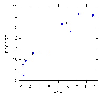
A multiple regression analysis was then carried out, with D-score as
the dependent variable and both BOY and AGE as independent variables.
The results are shown in Table 2. This time the effect of BOY
becomes non-significant (P-value is 0.799); the effect of AGE on D-score
is strongly significant. One concludes that the significant effect
of sex (represented by the variable BOY) in the first regression was spurious.
It was a consequence of the (accidental) association in the sample between
age and sex, i.e. the tendency (visible in the scatterplot) for boys to
be older than girls, combined with the strong effect of age on D-score.
Introducing ("controlling for") age in the model has eliminated the spurious
effect of sex on cognitive development.
Table A2. Multiple Regression of D-Score on BOY and AGE
Dep Var: DSCORE
N: 12 Multiple R: 0.958 Squared multiple R: 0.917
Adjusted squared multiple
R: 0.899 Standard error of estimate: 0.634
Effect
Coefficient Std Error Std Coef
Tolerance t P(2 Tail)
CONSTANT
6.927 0.506
0.000 . 13.697
0.000
BOY
-0.126 0.480
-0.033 0.581 -0.262
0.799
AGE
0.753 0.097
0.979 0.581 7.775
0.000
Analysis of Variance
Source
Sum-of-Squares df Mean-Square
F-ratio P
Regression
40.002 2 20.001
49.765 0.000
Residual
3.617 9
0.402
-------------------------------------------------------------------------------
Durbin-Watson D Statistic
2.277
First Order Autocorrelation
-0.313
Appendix B. Standard Tabular Presentation of Regression Results
1. Standard Presentation
The standard journal presentation of multiple regression results is aimed
in part at facilitating the elaboration model by examining the effect of
introducing a new "test" variable in the model.
The following table presents the results of the regression analysis
of the D-score data in standard tabular format.
Table B1. Unstandardized Regression Coefficients of Cognitive
Development (D-score) on Sex and Age for 12 Children Aged 3 to 10 (t Ratios
in Parentheses)
| Independent variable |
Model 1
|
Model 2
|
| Constant |
10.305***
|
6.927***
|
| |
(15.109)
|
(13.697)
|
| Boy ( boy=1, girl=0) |
2.288*
|
-.126
|
| |
(2.372)
|
(-.262)
|
| Age (years) |
--
|
.753***
|
| |
|
(7.775)
|
| R2 |
.360
|
.917
|
| Adjusted R2 |
.296
|
.899
|
| Note: * p < .05 ** p < .01 ***
p < .001 (2-tailed tests) |
2. Suggestions on Preparing Tables of Regression Results
The following guidelines would help prepare tables of results acceptable
by most professional journals.
-
the title of the table contains information on the type of regression coefficients
shown (here, unstandardized coefficients), the dependent variable, the
independent variables (when there are too many to list in the title, one
says "on selected independent variables"), the nature of the units of observation
(children in a given age range), and the sample size (12). When n
is not the same in all the models (e.g., because of missing data), state
the maximum n in the title and specify the actual sample sizes in a row
labeled "N" placed below "Adjusted R-square". When appropriate, add
to the title information on elements of the larger context, such as geographic
location and time frame.
-
the independent variables are introduced one at a time in successive models
shown in the different columns of the table; variants of this strategy
often introduce together sets of related variables, such as
-
a set of indicators representing a categorical variable
-
different powers of X representing a polynomial function
-
variables related conceptually, e.g. father's education, mother's education,
and family income together representing family SES
-
significance levels of the coefficients are indicated with asterisks. American
Sociological Review usage is shown here. Check the main journals
in your field for usage. A legend at the bottom of the table indicates
the meaning of the symbols and specifies the type of test used (1-tailed
or 2-tailed). Both 2-tailed and 1-tailed tests can be used in the
same table by using a different symbol for 1-tailed tests. EX:
add a line at the bottom with: + p < .05 ++ p < .01 +++
p < .001 (1-tailed tests)
-
both R-square and Adjusted R-square are shown. Reviewers will often
insist that you show the adjusted R-square, even though N may be so large
it makes no difference. Give it to them. Never omit the regular
("unadjusted") R-square, though, as this can be used to reconstruct F-tests
from the table more easily (see Module 8)!
-
the t-ratios (coefficient estimates divided by their standard error) are
shown in parentheses below the regression coefficients. Some people
present the standard error instead of the t-ratio, but this is a deplorable
practice because the standard errors are in the metric of the corresponding
regression coefficients. Thus standard errors are in general not
comparable across coefficients (unless the independent variables are in
the same metric) and they suffer different degrees of rounding when a fixed
number of decimal places is used. Because of this t-ratios for some
coefficients may not be computable with sufficient precision from the table,
which may lead to incorrect judgements of significance. By contrast
t-ratios are all in the same metric (that of a Student t variate with n-p
df) and are therefore directly comparable across coefficients, and they
convey the same (optimal) degree of precision across all coefficients when
a fixed number of decimals is used. Thus it is much better to
present the t-ratios than the standard errors of estimate.
-
a place holder (--) is used in place of the regression coefficient to show
that a variable is not included in a model; this is especially helpful
in large tables with many columns
-
the independent variables are labeled with human readable text, not the
computer symbol, in such a way that
-
the name of the variable is consistent with the numerical scale (e.g.,
SES must have values that are large for high SES and small for low SES;
values of "Democracy" must be high for democratic countries and low for
non-democratic ones)
-
the coding of a 0,1 indicator variable is explicitly defined when any doubt
is possible (e.g., an indicator called SEX must specify whether it is coded
as 1 for male and 0 for female, or the other way around)
-
the best way to label an indicator variable is with the name of the category
that is coded 1 (e.g., instead of calling the indicator SEX or GENDER,
call it MALE (with 1 for male and 0 for female) or FEMALE
(with 1 for female and 0 for male)
Appendix C. Multiple Regression in Practice
Instructions to do multiple regression with a variety of options are provided
in the following exhibits.
Last modified 6 Mar 2006
![Exhibit: George Udny Yule (1871-1951) (1) [Yule.jpeg]](../odocs/Yule.jpg)
![Exhibit: George Udny Yule (1871-1951) (2) [Yule_2.jpeg]](../odocs/Yule_2.jpg)
![Exhibit: Quote from Yule (1899, p. 251) [m5003a.gif]](m5003a.gif)
![Exhibit: Yule's original regression results (Yule 1899, Table C p. 259) [m5004a.gif]](m5004a.gif)
![Exhibit: The mechanism of spuriousness/specification bias [m5003.gif]](m5003.gif)
![Exhibit: Cross-national model of income inequality (Nielsen 1994 Table 3 p. 670) [m5006.gif]](m5006.gif)